
Download

MAD v1 1995 application screenshot
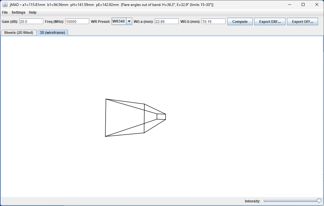
jMAD application screenshot
What jMAD Does
Goal Compute a rectangular pyramidal horn directly from a target gain and waveguide back section, using a closed set of relations that start with Jasik’s directivity formula and collapse to a single nonlinear variable (chi = l_e λ). jMAD solves this horn-design equation via Newton–Raphson, then generates manufacturing geometry (plate outlines) and exports DXF (R2000/LWPOLYLINE) that most 2D CAM systems accept. rectangular pyramidal horn
Jasik’s classic treatment gives a rectangular pyramidal horn’s directivity in terms of the E‑plane and H‑plane slant lengths, (l_e) and (l_h):
D = (4π/λ²) · √(3 l_h λ) · √(2 l_e λ)
The constants √3 and √2 reflect the rectangular aperture weighting in the H- and E-planes. This formula and its context appear in the classic Antenna Engineering Handbook (Jasik) and in many university notes that derive pyramidal horn geometry from sectoral-horn approximations.
2) Equal-slant requirement and phase-deviation consistency
In fabrication, all four horn sheets must meet cleanly at the aperture, so we enforce an equal-slant condition (l_e = l_h) for a rectangular horn that transitions from a rectangular waveguide back (internal dimensions (a, b)) to a rectangular aperture ((a_1, b_1)). Combining Jasik’s sectoral relations with the equal-slant constraint and a phase-deviation (aperture phase error) consistency yields a single horn-design equation in the dimensionless variable (chi equiv l_e λ). (The phase-deviation consistency follows the Schelkunoff/Jasik line; several modern notes present equivalent constraints.)
3) My UTas (Australian Maritime College) χ-substitution and the horn-design equation
Using (chi = l_e λ) and normalizing the back waveguide dimensions by the wavelength, (A equiv a λ), (B equiv b λ), the horn-design equation becomes:
( √(2χ) − B )² · (2χ − 1)
  − ( G /(2π) ) · ( √( (2/(2π)) · 1/√χ ) − A )² · ( (G²)/(6π³) · 1/χ − 1 )  =  0
Here, (G) is the dimensionless target gain (not in dB). In practice we often work with a target gain and an aperture efficiency (η) so that the design uses directivity \(D = Gη). (jMAD exposes (η) as a menu setting; by default (η) is ~0.6–0.8 for pyramidal horns.)
4) Newton–Raphson solution
We solve ( f(χ) = 0 ) (the equation above) by Newton–Raphson:
// Seed (a sensible starting point):
χ₀ = G / (8 π³)

// Iterate:
repeat
  χ ← χ − f(χ)/f′(χ)
until |Δχ| < ε  and  χ > 0.5
Guarding (χ > 0.5) ensures the factor ((2χ-1)) remains positive in the geometry. A derivative (f′(χ)) can be carried analytically to improve stability and speed. For extreme parameters, a bracketed fallback (bisection) ensures robustness.
5) From (χ) to physical dimensions
Once (χ) is found:
l_e = l_h = χ λ
a₁ = √(3 λ l_h)
b₁ = √(2 λ l_e)

// Axial lengths from simple right-triangle geometry:
p_H = √( l_h² − ((a₁ − a)/2)² )
p_E = √( l_e² − ((b₁ − b)/2)² )
These give you the **aperture** ((a_1, b_1)) and the **H/E axial plate lengths** ((p_H, p_E)) directly from the solution (χ). The outlines of the four plates are then isosceles trapezoids (TOP/BOTTOM: H‑plane; LEFT/RIGHT: E‑plane), offset about the back section for symmetric flare.
6) Practical flare-angle guardrail
Define full flare angles:
θ_H = 2 arctan( (a₁ − a)/(2 p_H) )
θ_E = 2 arctan( (b₁ − b)/(2 p_E) )
In practice, designers keep horn flares within a moderate band—often quoted around ~15°–30°—to limit spherical expansion loss and excessive aperture phase error. jMAD flags out‑of‑range angles; the limits are user‑adjustable. (Exact “optimum” limits depend on taper/phase assumptions and application.)
Design Workflow (step by step)
- Choose WR back section (internal (a, b)) from the presets (e.g., WR90 = 22.86 mm × 10.16 mm). [2](https://www.pdfagile.com/blog/a3-paper-size)
- Set frequency (f) (MHz) → wavelength (λ ≈ 300/f) (m).
- Enter target gain \(G_{dB}\) and aperture efficiency (η) → directivity (D = 10^{G_{dB}/10} / η).
- Solve (f(χ)=0) (above) with Newton–Raphson, seed (χ_0 = G/(8π^3)).
- Compute ((a_1, b_1, p_H, p_E)); check (θ_H, θ_E) vs. your limit band.
- Export DXF for TOP/BOTTOM/LEFT/RIGHT plates (LWPOLYLINE, closed). [1](https://storage.googleapis.com/duehbtgqsaapwe/horn-antenna-dimensions.html)
Program Details
- Solver: Newton–Raphson on (χ) with analytic derivative and bracketed fallback.
- Efficiency (η): Adjustable; the design uses (D = G/η) internally.
- WR presets: Common WR dimensions (a×b) from standard tables. [2](https://www.pdfagile.com/blog/a3-paper-size)
- DXF export: ASCII R2000/AC1015 with LWPOLYLINE entities (closed). Most R14/2000 CAMs import this directly. [1](https://storage.googleapis.com/duehbtgqsaapwe/horn-antenna-dimensions.html)
File Format Notes
| Format | What jMAD writes | Why it’s chosen |
|---|---|---|
| DXF | R2000 (AC1015) header; LWPOLYLINE entities; closed plates per layer | Lightweight polylines are compact and widely compatible with R13/R14/2000‑era tools. [1](https://storage.googleapis.com/duehbtgqsaapwe/horn-antenna-dimensions.html) |
References
- Jasik, H. (ed.), Antenna Engineering Handbook (classic editions). Archive record: Internet Archive – Antenna Engineering Handbook.
- Standard WR dimensions (example: WR90 = 22.86 mm × 10.16 mm): RF Wireless World – WR size chart. [2](https://www.pdfagile.com/blog/a3-paper-size)
- AutoCAD DXF LWPOLYLINE group codes: Autodesk Help – LWPOLYLINE (DXF). [1](https://storage.googleapis.com/duehbtgqsaapwe/horn-antenna-dimensions.html)
Credits
jMAD – by Gregory J. Durnan, 2026.
Website: durnan.org