Downloads
This little workbench started life in the most dangerous of places: an Excel spreadsheet that “looked right” until the physics politely disagreed. What you’ll find here is the cleaned-up, Java-based evolution of that experiment: a finite-difference model of a 2D birdcage coil, solving for the magnetic vector potential and visualizing the resulting B fields in several ways.
From Spreadsheet to Workbench
The original model was a scalar-potential FDM in Excel. It was a great sandbox, but it quietly assumed an electrostatic world: charges, not currents; gradients, not curls. Once the goal shifted to modeling an MRI-style birdcage coil, the physics demanded an upgrade:
- Switch from scalar potential φ to magnetic vector potential Az for current-driven fields.
- Introduce Neumann / absorbing boundary conditions by “folding” the edges of the grid.
- Increase the matrix size so the boundaries stop bullying the solution in the center.
The result is this Birdcage FDM Workbench: a 1000×1000 grid, adjustable birdcage diameter and rung count, multiple visualizations, and just enough UI polish to make it fun to poke at.
Theoretical Background – Finite Differences in a Birdcage
1. The core PDEs
Electric (scalar) formulation:
∇²φ = -ρ / ε
E = -∇φ
Magnetic (vector) formulation (used here):
∇²A = -μ₀ J
B = ∇ × A
In this workbench we assume a 2D cross-section with currents flowing along z, so only Az(x, y) is non-zero. That collapses the vector Poisson equation into a scalar Poisson equation in Az, but the physics is still magnetic: the sources are currents, not charges, and the field we care about is B, not E.
2. Discretizing the Laplacian
On a uniform grid with spacing Δx = Δy = DX, the 2D Laplacian becomes:
∇²A_z(i,j) ≈ [A_z(i+1,j) + A_z(i-1,j) + A_z(i,j+1) + A_z(i,j-1) - 4 A_z(i,j)] / DX²
The discrete Poisson equation at each interior node is:
A_z(i+1,j) + A_z(i-1,j) + A_z(i,j+1) + A_z(i,j-1) - 4 A_z(i,j) = -μ₀ J_z(i,j) DX²
We solve this iteratively using SOR (Successive Over-Relaxation), updating Az until it settles into a self-consistent solution that satisfies the PDE and the boundary conditions.
3. From Az to B and |B|
With only Az non-zero, the magnetic field is:
B_x = ∂A_z / ∂y
B_y = -∂A_z / ∂x
Using central differences:
B_x(i,j) ≈ [A_z(i, j+1) - A_z(i, j-1)] / (2 DX)
B_y(i,j) ≈ -[A_z(i+1, j) - A_z(i-1, j)] / (2 DX)
|B|(i,j) = sqrt(B_x² + B_y²)
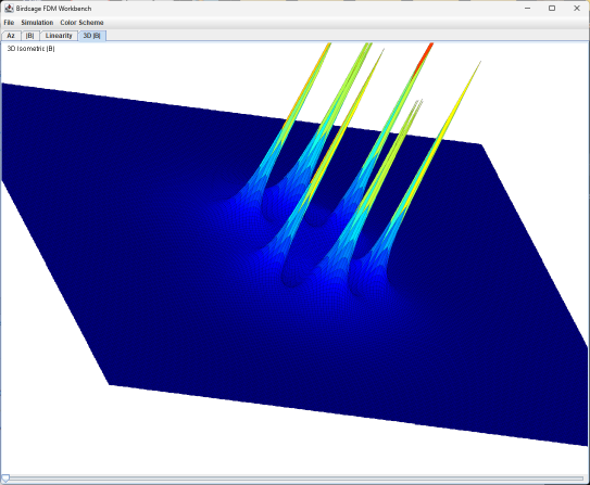
This is what you see in the |B| tab and the 3D |B| surface: the magnitude of the curl of Az, sampled across the grid.
Electric vs Magnetic FDM – What Really Changes?
| Aspect | Electric FDM (Scalar φ) | Magnetic FDM (Vector A) |
|---|---|---|
| Unknown | Scalar potential φ(x, y) | Vector potential A(x, y), here reduced to Az(x, y) |
| Source term | Charge density ρ | Current density Jz along the rungs |
| Field recovery | E = -∇φ (gradient) | B = ∇ × A (curl) |
| Typical boundaries | Dirichlet (fixed φ), Neumann (insulating) | Neumann / absorbing (open space), sometimes Dirichlet on PECs |
| Geometry sensitivity | Charges are points/volumes | Currents live on paths (rungs, loops) |
| Angular structure | Often not critical | Essential – birdcage modes are cosine/sine around the ring |
| “Feels wrong” failure mode | Potential looks smooth but doesn’t match boundary physics | |B| looks distorted by boundaries or wrong current phasing |
Boundary Conditions, Nonlinearities, and “Why Is My Field So Weird?”
Neumann / ABC by folding the edges
A finite grid has edges; the real world doesn’t. If you simply clamp Az to zero at the boundary, you create an artificial conducting box that reflects fields back into the domain. The fix used here is a simple Neumann / absorbing boundary condition:
// top and bottom
Az[i][0] = Az[i][1];
Az[i][NY - 1] = Az[i][NY - 2];
// left and right
Az[0][j] = Az[1][j];
Az[NX - 1][j] = Az[NX - 2][j];
This “folds” the edges so the normal derivative is approximately zero, letting the field leave the domain without a dramatic bounce-back. It’s not a perfect ABC, but it’s simple, robust, and good enough for a birdcage playground.
Matrix size and the tyranny of boundaries
Early versions used a relatively small matrix. The birdcage looked fine, but the boundaries were so close that they warped the field in the center. The cure was simple but non-negotiable:
- Make the matrix big (1000×1000).
- Automatically choose DX so the birdcage diameter is ≤ 1/4 of the grid width.
Once the coil is comfortably “inside” the domain, the center region behaves like free space and the |B| pattern finally looks like the physics textbooks promised.
Iterative solvers and the art of “try, fix, repeat”
The whole project is a nice reminder that finite-difference modeling is inherently iterative in two senses:
- Numerically: SOR iterates the solution until it converges.
- Conceptually: you iterate the model itself – potentials, boundaries, grid size – until the physics and numerics agree.
The first Excel version “worked” in the sense that it produced numbers and pretty colors. The Java workbench works in the sense that the fields are physically meaningful, stable, and interpretable. The gap between those two is where all the learning happened.
What the Workbench Shows You
- Az tab: The magnetic vector potential Az across the grid.
- |B| tab: The magnitude of the magnetic field derived from Az.
- Linearity tab: A central line cut of |B|, normalized, to see homogeneity.
- 3D |B| tab: A rotatable 3D surface of |B| with shading and contour-like edges.
You can change the number of rungs, adjust the birdcage diameter, switch color maps, export OFF geometry, and save PNGs of any view. Under the hood, it’s still just finite differences on a grid – but with enough knobs to make the physics visible and the trade-offs tangible.