jMiniNEC — The Math Behind a 1984 NOSC Antenna Solver, Ported Line-by-Line Into Java
I promised myself I'd go deep this time. Elsewhere on this site is the fun, breezy version of "here's some old-school MoM code and roughly what it does." This isn't that. This is the actual mathematics underneath MININEC — specifically, my MININEC: the QB45 program I wrote in the early 1990s, recently reworked in QB64, and now ported — procedure for procedure, bug for bug (well, three bugs fewer than before) — into a clean, headless Java class I'm calling jMiniNEC.
A quick scoping note before we start, because MININEC has a complicated family tree and I don't want to promise more than this code delivers. There's a "full" MININEC(3) — the 1986 NOSC Technical Document 938 version, by Logan and Rockway — that supports lossy real ground via Fresnel reflection coefficients, dielectric constant, conductivity, ground screens, near-field probes, the works. That is not what's in this article. My QB45 program is a leaner descendant, closer to the original 1980 MININEC (NOSC TD 516, Julian, Logan and Rockway) plus a perfect-image ground option. No Sommerfeld integrals, no lossy earth, no ground screens. Just: wire segments, a thin-wire kernel, a pulse basis, point matching, and a matrix you invert. That simplicity is exactly why it fit in a few hundred lines of BASIC on a machine with less memory than this paragraph.
Where This Code Actually Comes From
MININEC was written at the Naval Ocean Systems Center in San Diego — NOSC, not to be confused with the present-day Navy Operational Support Centers scattered around the country, which are Navy Reserve admin offices with nothing to do with antennas. The MININEC NOSC was a genuine electromagnetics research lab, formed March 1, 1977 from the merger of the Naval Electronics Laboratory Center and the Naval Undersea Center, and it existed under that name until the early 1990s, when a run of Navy lab consolidations eventually folded its work into what is today the Naval Information Warfare Center Pacific.
The original reference is A. J. Julian, J. C. Logan and J. W. Rockway, MININEC: A Mini-Numerical Electromagnetics Code, NOSC Technical Document 516 (1980). It's the program my QB45 code's own banner credits — "REFERENCE-JULIAN ET AL, NOSC TD 516" — which is a nice thing to be able to confirm forty-some years later. The idea was refreshingly practical for its era: NEC (the Numerical Electromagnetics Code) was — and still is — the serious, comprehensive tool for this kind of problem, but it needed a mainframe. MININEC was NEC's method stripped down hard enough to run in BASIC, on a microcomputer, in the field. "Mini" is doing real work in that name.
The Physics: Pocklington's Equation, Sort Of
Every thin-wire MoM code starts in the same place: Maxwell's equations, a thin perfectly-conducting wire, and the boundary condition that the tangential electric field must vanish on the wire's surface. Pocklington worked this out in 1897; MININEC uses a form of the same idea, but expressed through the vector and scalar potentials rather than Pocklington's differentiated kernel directly — which turns out to matter a lot for how cheaply you can compute it.
The vector potential \(\bar{A}\) and scalar potential \(\phi\) along the wire are
\[ \bar{A} = \frac{\mu}{4\pi} \int_c I(s')\,\hat{s}(s')\,k(s-s')\,ds', \qquad \phi = \frac{1}{4\pi\varepsilon} \int_c q(s')\,k(s-s')\,ds', \]where \(q(s)\) is the linear charge density, related to the current by the continuity equation \(q(s) = -\frac{1}{j\omega}\frac{dI}{ds}\), and \(k(s-s')\) is the thin-wire kernel
\[ k(s-s') = \frac{1}{2\pi}\int_{-\pi}^{\pi} \frac{e^{-jkr}}{r}\,d\phi, \qquad r = \left[(s-s')^2 + 4a^2\sin^2\tfrac{\phi}{2}\right]^{1/2}, \]averaging the exact free-space Green's function around the wire's circumference (radius \(a\)) so the whole problem stays one-dimensional — a function of arc length \(s\) along the wire axis, not a full 2-D surface integral. That averaging is the "thin-wire approximation," and it's the single assumption that makes MININEC (and NEC, and every code like it) tractable at all.
The field equation that ties all this together is
\[ -\bar{E}_{inc}\cdot\hat{s} = -j\omega\bar{A}\cdot\hat{s} - \hat{s}\cdot\nabla\phi , \]which just says: the incident tangential field along the wire is balanced by the tangential vector-potential term (the "inductive" part) and the gradient of the scalar potential (the "capacitive" part). Everything from here is about how you turn that one equation — still exact, still continuous, still unsolvable by hand for anything interesting — into \(N\) linear equations in \(N\) unknown currents.
Chopping the Antenna Into Pulses
MININEC discretizes with the simplest basis function there is: a pulse. The wire is cut into \(N\) equal segments, and the current on segment \(n\) is assumed constant — one complex number per segment. Formally,
\[ I(s) = \sum_{n=1}^{N} I_n P_n(s), \qquad P_n(s) = \begin{cases} 1, & s_{n-1/2} < s < s_{n+1/2} \\ 0, & \text{otherwise} \end{cases} \]where the \(s_{n\pm 1/2}\) are segment midpoints. Testing ("point matching," or collocation) then enforces the field equation only at each segment's own midpoint, rather than trying to satisfy it everywhere at once. That's a Galerkin-adjacent shortcut — test with the same pulse functions you expanded with — and it's exactly what makes the resulting matrix equation cheap to fill: one integral per matrix entry instead of a double integral.
There's a subtlety in how the charge is represented, though, that doesn't show up if you only think about the current. Because \(q(s)\) is a derivative of \(I(s)\), and \(I(s)\) is a staircase of pulses, its derivative is a train of impulses at the segment boundaries — so MININEC represents charge as a second set of pulses, the same width as the current pulses but shifted by half a segment. Current pulses sit on segment junctions; charge pulses sit on segment centers. This half-segment offset between the two pulse families is why so much of the kernel code below is written in terms of "P1 ± 0.5" style segment arithmetic — it isn't decoration, it's the charge representation leaking into the indexing.
This scheme also has to handle the ends of wires and the junctions between them. A wire with a free end just omits the pulse there — equivalent to forcing a zero-amplitude half pulse, which enforces zero current at an unconnected tip, exactly as physics demands. A junction of two or more wires is handled by overlapping pulses: the last full pulse of one wire is allowed to straddle into the next wire, with Kirchhoff's current law satisfied automatically because the overlapping pulse's amplitude is shared between both wires' equations. It's a clever bit of bookkeeping that avoids ever writing down an explicit continuity constraint.
Here's that bookkeeping as it survives in the Java port, straight out of defineWire() — computing
a wire's direction cosines and figuring out where its pulses land in the shared coordinate arrays:
// direction cosines (unit vector along the wire) and per-segment length
x3 = x2 - x1;  y3 = y2 - y1;  z3 = z2 - z1;
d = Math.sqrt(x3 * x3 + y3 * y3 + z3 * z3);
dArr[wireIndex] = x3 / d;   // D(I): x-direction cosine
fArr[wireIndex] = y3 / d;   // F(I): y-direction cosine
gArr[wireIndex] = z3 / d;   // G(I): z-direction cosine
sArr[wireIndex] = d / s1;   // S(I): length of one segment

// how many NEW pulses this wire contributes, minus one at each free end
n1 = n + 1;
n = n1 + s1;
if (i1 == 0) n = n - 1;   // end 1 unconnected -> one fewer pulse
if (i2 == 0) n = n - 1;   // end 2 unconnected -> one fewer pulse

// C(*,1) / C(*,2): which wire each pulse's two half-segments belong to
for (j = n1; j <= n; j++) {
    cArr[ix(j)][1] = wireIndex;
    cArr[ix(j)][2] = wireIndex;
}
cArr[ix(n1)][1] = i1;   // overwritten with the connecting wire's number
cArr[ix(n)][2] = i2;    // (or left as +-wireIndex if this end is free/grounded)
That cArr/C() array is doing a lot of quiet work: by the time matrix fill runs, each
pulse knows which physical wire(s) it belongs to on either side, which is exactly the information the overlap
scheme above needs to enforce current continuity at junctions without ever solving a separate constraint
equation for it.
The Kernel's Dirty Little Secret
Here's the part that makes MININEC MININEC rather than just "NEC but smaller." Filling the impedance matrix means evaluating an integral of the kernel \(k(s-s')\) over each source segment, for each observation point:
\[ \int_{s_u}^{s_v} k(s-s')\,ds'. \]The trouble is \(k\) has a logarithmic singularity right where you need it most — the self term, where the observation point sits on top of the source segment (\(r \to 0\)). You can't just Gaussian-quadrature your way through that; the integrand blows up exactly at the point you're sampling.
MININEC's trick is to subtract the singularity out analytically, integrate the well-behaved remainder numerically, and add the analytic part back as a closed form. Split the kernel into three pieces,
\[ k(s_m - s') = -\frac{1}{\pi a}\ln\!\left[\frac{|s_m - s'|}{8a}\right] \;+\; \frac{\beta\,F(\tfrac{\pi}{2},\beta) + \ln\!\left[\frac{|s_m-s'|}{8a}\right]}{\pi a} \;+\; \frac{1}{2\pi}\int_{-\pi}^{\pi} \frac{e^{-jkr}-1}{r}\,d\phi , \]where the first term is the bare log singularity (integrated in closed form), the second is the difference between the exact near-field behavior — an elliptic integral of the first kind, \(F(\tfrac{\pi}{2},\beta)\) — and that same log singularity (smooth, no blow-up, safe to integrate numerically), and the third mops up everything else (also smooth). Add all three back together and the singularity has vanished without ever being approximated away.
The one wrinkle is that \(F(\tfrac{\pi}{2},\beta)\) itself is an elliptic integral, and nobody wants to evaluate a special function from scratch inside a 1980s BASIC interpreter for every matrix entry. So MININEC leans on a well-known rational-plus-log approximation,
\[ F\!\left(\tfrac{\pi}{2},\beta\right) \approx \left(a_0 + a_1 m + a_2 m^2 + a_3 m^3\right) \;-\; \left(b_0 + b_1 m + b_2 m^2 + b_3 m^3\right)\ln\!\left(\tfrac{1}{m}\right), \]with \(m = 1 - \beta^2\) and five fixed coefficients each for \(a\) and \(b\). This is a textbook
approximation (Abramowitz & Stegun-style), and MININEC just carries the ten constants as DATA in
the BASIC source. They land in the Java port's wArr field, and this is where all that near-field
correction machinery in gosub9() (the port's name for BASIC's TARGET9 subroutine) comes
from:
if (i6 != h0) {                                 // "near" case only
    d3 = pointDist * pointDist - a2;            // (a2 = wire-radius^2)
    b = d3 / (d3 + 4 * a2);                     // beta^2, roughly
    v1 = wArr[1]; v2 = wArr[6];                 // a0, b0
    b1 = 1; b2 = -36;
    for (l2 = 2; l2 <= 5; l2++) {                // accumulate a1..a4, b1..b4
        b2 = b2 / (l2 - 1);
        if (b < Math.pow(10, b2)) break;         // early-out once terms are negligible
        b1 = b1 * b;
        v1 = v1 + wArr[ix(l2)] * b1;
        v2 = v2 + wArr[ix(l2 + 5)] * b1;
    }
    v = (v1 - v2 * Math.log(b)) * Math.sqrt(1 - b);   // the F(pi/2, beta) approximation
    d3 = Math.sqrt(d3) / 8 / aArr[ix(p4)];
    t3 = t3 + (Math.log(d3) + v) / p / aArr[ix(p4)] - 1 / pointDist;
}DATA constants against the
original reference table turned up one that's slightly off: \(b_4\) should be 0.00441787012, but
the BASIC source has .0041787 — a transposed digit from forty-some years of copying a number by
hand, most likely. It's the smallest-order term in a five-term series that's already an approximation, in a
correction that only matters for the self and near terms, so the practical effect is somewhere south of
negligible — re-running the half-wave dipole case below with the corrected constant moves the feedpoint
impedance by about \(2\times10^{-5}\,\Omega\), four decimal places past anything reported here. I've
corrected it in wArr in jMiniNEC anyway, on the general principle that there's no reason to keep
carrying a known transcription error forward once you've found it, harmless or not. It's a fun thing to be
able to say with confidence forty years later, and it says something nice about how forgiving this
kind of numerical method is — one mistyped digit, five layers deep in an approximation to an approximation,
and the antenna still resonated exactly where it should the whole time.
Filling the Matrix
With the kernel integral in hand, each entry of the impedance matrix is
\[ Z_{mn} = \frac{-1}{4\pi j\omega\varepsilon} \Bigg[ k^2(\bar{r}_{m+1/2} - \bar{r}_{m-1/2})\cdot (\hat{s}_{n+1/2}\,\psi_{m,n,n+1/2} + \hat{s}_{n-1/2}\,\psi_{m,n-1/2,n}) - \cdots \Bigg], \]a combination of the scalar-potential integral \(\psi\) (the kernel integral from the previous section) and the direction-cosine dot products between the observation segment and the source segment. In plain terms: how strongly does current flowing along source segment \(n\) couple, via the retarded near/far-field kernel, into the tangential field MININEC is testing at segment \(m\).
That direction-cosine dot product shows up explicitly in the matrix-fill code, and it's worth seeing because it's such a direct translation of the vector algebra above:
// T5,T6,T7 = the observation segment's effective direction vector,
// combining the two half-segments either side of pulse I's junction
t5 = f5 * dArr[ix(i2)] + f4 * dArr[ix(i1)];
t6 = f5 * fArr[ix(i2)] + f4 * fArr[ix(i1)];
t7 = f5 * gArr[ix(i2)] + f4 * gArr[ix(i1)];
Ground handling is where MININEC's simplicity really pays off. For a perfectly conducting ground plane, image
theory says: replace the ground with a mirror-image copy of the whole wire structure, with currents related by a
known sign, and solve twice as many unknowns. A naive implementation really would double the matrix size.
MININEC's fill loop instead runs an inner K = 1 To G loop (G is 1 for free space, 2
for "near earth") that adds the image contribution straight into the existing \(N\times N\) matrix
entry, with a sign flip on the \(z\) component for the mirrored geometry, rather than ever assembling a literal
\(2N \times 2N\) system and reducing it back down. Same physics, half the memory, and it's why the ground flag is
a single BASIC Input statement rather than a dielectric constant and conductivity — there's no
lossy-ground term anywhere in this code path, just a mirror image.
Solving It: Gaussian Elimination, in Complex Arithmetic
Once \([Z_{mn}][I_n] = [V_m]\) is filled, someone has to invert it. This code does the direct, 1984 thing —
in-place Gaussian elimination with pivoting, operating on parallel real and imaginary matrices
(R()/B() in the original, rArr/bArr here) since BASIC of
that era had no native complex type.
One thing worth calling out: the pivot search isn't just partial (largest entry in the current column) — it searches the entire remaining unreduced submatrix, rows and columns both, for the largest-magnitude entry, and swaps that into position:
for (int jj = ix(h0); jj <= nn; jj++) {
    if (pArr[jj] == h0) continue;                 // already used as a pivot row
    for (int kk = ix(h0); kk <= nn; kk++) {
        if (pArr[kk] == h0) continue;              // already used as a pivot column
        s2 = rArr[jj][kk] * rArr[jj][kk] + bArr[jj][kk] * bArr[jj][kk]; // |Z|^2
        if ((s1 - s2) > 0) continue;
        i1 = jj; i2 = kk; s1 = s2;                 // new best pivot candidate
    }
}
That's closer to complete pivoting than the row-only partial pivoting most textbooks teach — a nice
bit of numerical conservatism for code meant to run unattended on borrowed computer time, where a
badly-conditioned matrix silently returning garbage would be far worse than the extra \(O(N^2)\) search cost per
elimination step. After the pivot is found and swapped in, the elimination itself is the standard complex
generalization of the real algorithm — divide the pivot row by the pivot element (using complex reciprocal,
computed by hand as \((a - bi)/(a^2+b^2)\) since again, no native complex type), then subtract multiples of it
from every other row. P() (pArr here) tracks which rows/columns have been consumed as
pivots; H()/I() record the pivot history so the solution can be unscrambled back into
the original row order once elimination finishes.
Radiating It Out
The last stage turns the solved current distribution into a far-field radiation pattern. For a set of pulse currents \(I_n\), the far electric field in direction \((\theta,\phi)\) is (dropping constants that don't depend on direction)
\[ \bar{E}(\bar{r}_0) \propto \sum_{n} I_n\, \big[(\hat{k}\cdot\hat{s}_n)\hat{k} - \hat{s}_n\big]\, e^{\,j\bar{K}\cdot\bar{r}_n}, \]a sum, over every current pulse, of that pulse's contribution weighted by its phase relative to the observation direction \(\hat{k}\). Each wire segment's contribution factors into a magnitude term (essentially sinc-shaped, from integrating a constant current over a finite segment length) and a progressive phase term from \(\bar{K}\cdot\bar{r}_n\) — and both survive intact in the port:
// one pulse's contribution to the far-field sum
o = -(r1 * dArr[lIdx] + r2 * fArr[lIdx] + r3 * gArr[lIdx]) * f3v;
s1 = w * sArr[lIdx] / 2;
if (Math.abs(o) < .0000001) {
    o = (2 - o * o * s1 * s1 / 3) * s1;   // small-angle series: avoids 0/0
} else {
    o = 2 * Math.sin(o * s1) / o;          // the sinc-shaped element pattern
}
s2 = w * (xArr[pulseCoord] * r1 + yArr[pulseCoord] * r2 + zArr[pulseCoord] * r3);
s1 = Math.cos(s2);  s2 = Math.sin(s2);      // progressive phase, this pulse's position
b1 = (s1 * hArr[pulseI] - s2 * iArr[pulseI]) * o / f4v;   // complex multiply:
b2 = (s1 * iArr[pulseI] + s2 * hArr[pulseI]) * o / f4v;   // (current) x (phase) x (element pattern)
As with the impedance matrix, the ground-plane case doubles the summation (direct ray plus image ray) rather than doubling any array sizes — still nothing but perfect-conductor image theory. If you're the kind of person who wants Fresnel reflection off real, lossy dirt, that's MININEC(3) territory, not this code. I actually stumbled into exactly that distinction a while back cross-checking this port against an old help file that came with the original source, whose worked example uses real ground (dielectric constant 13, conductivity 0.005 S/m) — values this program never even asks for. Running the identical geometry through jMiniNEC with the perfect-image ground option gave a resistance within 0.2% of the help file's answer and a reactance within about 6%, which is exactly the kind of agreement you'd expect: close on resistance, off on reactance, because a perfect conductor and lossy real earth are similar but not identical grounds. Good sanity check; not a bug.
Does It Actually Work?
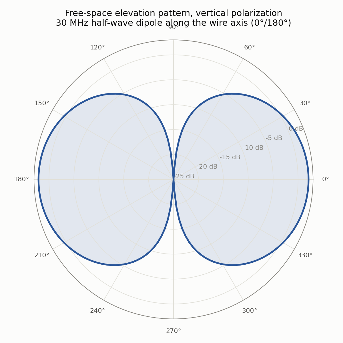
Talk is cheap in antenna theory, so here's the port actually running. A 30 MHz half-wave dipole, 10 segments, fed at the center pulse with 1 V:
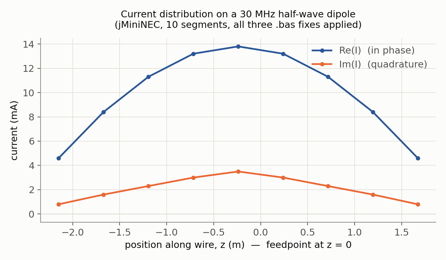
That's the current distribution you'd hope for and, for a while during this port, very much did not get — a smooth peak at the feedpoint, symmetric taper to (near) zero at both free ends. Getting here took finding and fixing three separate bugs in the 1984 BASIC itself, not just translation slips:
- a stray extra factor in the near-field kernel that NaN'd out any wire lying flat in a coordinate plane,
- a bare scalar used instead of an array lookup in the far-field phase term, and
- the subtle one: a single array slot doing double duty as both a wire's permanent direction cosine and the kernel's scratch space for a transient distance calculation, silently overwriting itself mid-computation.
All three are documented with exact original line numbers in the port's own comments, in case any of them ring a bell for the QB64 version too.
The radiation pattern above is the textbook half-wave dipole figure-8, broadside gain right around 2.1 dBi (the textbook value is 2.14 dBi for an idealized infinitely-thin half-wave dipole — close enough, given this one has a finite 1 mm radius and only 10 segments). Feedpoint impedance came out at \(67.71 - j17.35\,\Omega\), which is in the right neighborhood for a dipole that's a touch short of true half-wave resonance at this radius and segmentation.
I also cross-checked the raw impedance matrix — not just the final answer, the actual \(Z_{mn}\) entries —
against pymininec, an independent, actively maintained Python reimplementation of MININEC. For a
21.4 m wire at 7 MHz (a test case lifted straight from that project's own test suite), jMiniNEC's self term came
out \(-8.4796 - j0.009668\) against a reference of \(-8.4851 - j0.009669\), and the first off-diagonal term
\(4.2375 - j0.009573\) against \(4.2404 - j0.009573\) — agreement to three or four significant figures, with the
whole row decaying smoothly and monotonically the way a well-behaved thin-wire kernel should. That's about as
close to "provably correct" as a 1980s BASIC program is ever going to get.
Wrapping It Up
So that's the math: a thin-wire integral equation, tamed by a pulse basis and point matching; a kernel
singularity subtracted out with an elliptic-integral approximation that's been sitting in ten DATA
constants since 1984; a matrix filled by exploiting the ground plane as a doubled summation instead of a doubled
matrix; solved by a surprisingly careful complex Gaussian elimination; and radiated out through a closed-form
far-field sum. All of it small enough to have once run, slowly, on a machine that would struggle to render this
page today.
The full headless Java engine (no I/O, meant to be embedded) and its console-driver companion are available on request — too long to reprint here in full, in the spirit of keeping this page about the ideas rather than a code dump. If you want to see how a piece of 40-year-old Navy BASIC holds up when you port it faithfully, bugs and all, and then fix exactly the bugs that are provably bugs — this is that story.